I’m working on a project that needs non-contact detection. A few technologies fit — sonar, capacitive sensing, inductive sensing, and optical. Sonar and optical are out because of the enclosure, and capacitive sensing is too sensitive to temperature and humidity. That leaves inductive sensing. This post is my attempt to work through the principles. All data and designs are in the project repository.
Bit of Background#
The basic principle is the Self-Resonant Frequency (SRF) of the planar coil inductor (PCI). In practice, the coil isn’t a perfect inductor — parasitic capacitance and trace resistance are unavoidable. Calculating the SRF is pretty straightforward.
\[ SRF = \frac{1}{2\pi\sqrt{LC}} \]Where C is the total capacitance and L is the total inductance. The SRF shifts as you tweak either parameter.
When current flows through a trace, it induces a magnetic field around it. If the traces are arranged in a coil, those fields concentrate at the center.
When the field gets close to a conductive object like a copper sheet, it induces circular currents in the material — eddy currents. Just as current through a wire generates a field, those eddy currents generate their own, opposing the original. That’s Lenz’s Law. The opposing field reduces the effective inductance, shifting the SRF. That shift is the signal that something conductive is near the coil.
Inductance has two components, self-inductance and mutual inductance, which I’ll discuss below.
Mutual Inductance#
I’ll try to explain this without going too deep. By Lenz’s Law, when magnetic flux from one loop (A) passes through a second loop (B), the ratio of that flux \(\Phi_B\) to the current \(I_A\) in loop A is the mutual inductance \(M_{BA}\). The relationship is symmetric: \(M_{BA} = M_{AB}\).
\[ M_{BA} = \Phi_B /I_A \]This is given by the Neumann formula [1].
\[ M_{ij} = \frac{\mu_0R_iR_j}{2} \int_{\theta=0}^{2\pi} \frac{cos\theta}{\sqrt{R_i^2+R_j^2+d^2-2R_iR_jcos\theta}}d\theta \]Where:
- \( R_i, R_j \): Average radius of \(i^{th}\) and \(j^{th}\) loop between coil x and y, respectively
- \( d \): Distance between coils
This method is computationally heavy. A 4-layer board with 15 turns per layer means computing mutual inductances between every pair of turns on different layers — 1350 pairs, each a numerical integration from 0 to 2\(\pi\). Instead, I’ll use a simpler approximation that gives a constant coupling coefficient between two inductors.
\[ M_{12} = K\sqrt{L_1L_2} \]The K approximation is defined by the following paper [2]
\[ K = \frac{N^2}{0.64[(0.184x^3 - 0.525x^2 + 1.038x + 1.001)(1.67N^2 - 5.84N + 65)]} \]Where
- x: Distance between layers in mm
- N: Number of turns in the layer
Self Inductance#
Because the inductor is made up of consecutive loops, self-inductance can be explained much like mutual inductance. The flux from each loop passes through the others. By Faraday’s Law, that flux induces a current that opposes the incoming current. When the coil is flattened into two dimensions, its self-inductance can be approximated with the equation below [3]
\[ L = \frac{\mu_0N^2D_{avg}C_1}{2}(ln(\frac{C_2}{\sigma})+C_3\sigma+C_4\sigma^2) \]\[ \sigma = \frac{D_{outer} - D_{inner}}{D_{outer} + D_{inner}} \]Where:
- \( \mu_0 \): Free space permeability
- \( N \): Number of turns
- \( D_{avg} \): Average diameter of coil
- \( \sigma \): Fill factor
- \( C_1, C_2, C_3, C_4 \): Geometric coefficients [3]
Series Configuration#
Applying Kirchhoff’s Voltage Law to a string of inductors in series, with mutual inductance included, gives a simple summing equation similar to resistors in series. If the inductors are wound so the induced fields point in the same direction, the mutual inductances add.

The total effective inductance \(L_{eff}\) is the sum of the self-inductances \(L_a, L_b\) and the mutual inductances \(M_{ab}, M_{ba}\).
Parallel Configuration#
In the parallel case, I find it easier to use a system of equations to define the two branch voltages.
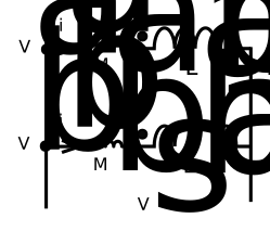
The node voltages \(V_a, V_b\) are sums of voltages across inductors \(L_a, L_b\) and their mutual inductances \(M_{ab}, M_{ba}\). Since \(V_a = V_b\) and assuming the inductors are identical, we can reduce the equations above to:
\[ L_{p\_eff} = \frac{L_aL_b-M^2}{L_a+L_b-2M}\]The point of parallel wiring isn’t to increase inductance — it’s to lower the resistance compared to a coil with similar physical dimensions, which makes for a more efficient drive circuit.
Planar Coil Inductor Layout#
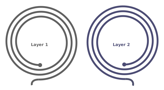
As mentioned, total inductance has two parts: self and mutual. For the coils to couple correctly, the winding direction has to flip on each subsequent layer.
Trace Resistance#
Trace resistance is reasonably straightforward. The trace length per layer is the arc length of an Archimedean spiral \(r(\theta) = r_0 + b\theta\), where \(r_0\) is the inner radius and \(b = p/(2\pi)\) is the radial growth per radian for pitch \(p\) (trace width plus trace-to-trace spacing). The exact arc length involves \(\sqrt{r^2 + (dr/d\theta)^2}\) in the integrand, but for typical PCB coils \(b \ll r_0\), so the approximation below is accurate to well under a percent:
\[ l \approx \int_{0}^{2n\pi} r(\theta)\,d\theta = 2\pi n r_0 + \pi n^2 p \]Where:
- \( l \): Trace length
- \( n \): Number of turns
- \( r_0 \): Inner radius
- \( p \): Pitch (trace width + spacing)
Then the trace resistance is:
\[ R_{DC} = \rho\frac{L}{T*W} \]Where:
- \( \rho \): Resistivity (copper ≈ 17.1×10⁻⁶ Ω·mm)
- \( L \): Length [mm]
- \( T \): Thickness (1 oz copper, 0.018–0.035 mm)
- \( W \): Width
Circuit Capacitance#
Because the resonant frequency depends on both inductance and capacitance, a small fluctuation in an already small parasitic capacitance can shift the resonant frequency significantly. So we want a sensor capacitor much larger than the unknown parasitic capacitance, to keep parasitic fluctuations from masquerading as inductance changes.
Assume a parasitic capacitance of 1 pF, a parallel sensor capacitor of 10 pF, and a nominal inductance of 10 µH. A 50% fluctuation in the parasitic capacitance shifts the apparent inductance by about 5%. With a 1 nF sensor capacitor, the same 50% fluctuation shifts the apparent inductance by less than 0.01%.
| Sensor C [F] | Parastic C [F] | Nominal L [H] | Resonant F [Hz] | Equivalent L [H] | Percent Change [%] |
|---|---|---|---|---|---|
| 10.000E-12 | 1.000E-12 | 10.000E-06 | 15.175E+06 | 10.000E-06 | 0.000 |
| 10.000E-12 | 1.100E-12 | 10.000E-06 | 15.106E+06 | 10.091E-06 | 0.909 |
| 10.000E-12 | 1.500E-12 | 10.000E-06 | 14.841E+06 | 10.455E-06 | 4.545 |
| 10.000E-12 | 900.000E-15 | 10.000E-06 | 15.244E+06 | 9.909E-06 | -0.909 |
| 10.000E-12 | 500.000E-15 | 10.000E-06 | 15.532E+06 | 9.545E-06 | -4.545 |
| 1.000E-09 | 1.000E-12 | 10.000E-06 | 1.591E+06 | 10.000E-06 | 0.000 |
| 1.000E-09 | 1.100E-12 | 10.000E-06 | 1.591E+06 | 10.001E-06 | 0.010 |
| 1.000E-09 | 1.500E-12 | 10.000E-06 | 1.590E+06 | 10.005E-06 | 0.050 |
| 1.000E-09 | 900.000E-15 | 10.000E-06 | 1.591E+06 | 9.999E-06 | -0.010 |
| 1.000E-09 | 500.000E-15 | 10.000E-06 | 1.591E+06 | 9.995E-06 | -0.050 |
Table 1: Effects of parasitic capacitance on effective inductance
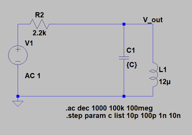
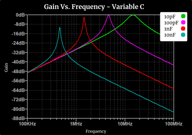
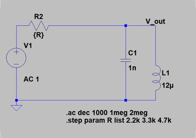
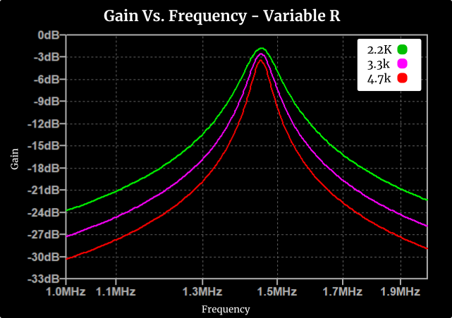
On the other hand, you can’t just drop in a 1 µF capacitor and be done. The more capacitance you add, the more high-frequency energy gets shunted away, lowering the bandwidth. In the figure below, at 1 nF, the gain at the resonant frequency is around -1.7 dB — for every volt in, 822 mV comes out. Easily measurable.
To approximate the system better, I’ll approximate the parasitic capacitance too. There’s a voltage gradient across the PCI — source voltage at the input, ground at the output — so I’m modeling it as two long parallel plates spiraled in a coil.
\[ C = \frac{\epsilon * w * l}{d}\]Where
- \(\epsilon\) is the relative electric permeability of the FR4 material (~4.4)
- w is the trace width
- l is the trace length per layer
- d is the thickness of the FR4 material
Validation#
To check my math, I’m using the Texas Instruments online coil designer tool [5]. It can’t approximate a PCI wired in parallel, unfortunately. Below are comparison results for the calculated inductor value, parasitic capacitance, resonant frequency, and trace resistance — a small subset of the data; the complete database is here.
The coil ID encodes its physical dimensions.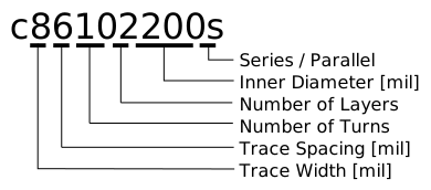
Inductor approximation#
| Coil Name | Self L Approximation | Total L Approximation | TI Self L | TI Total L | Total L Error |
|---|---|---|---|---|---|
| C106102200s | 1.349E-06 | 4.069E-06 | 1.110E-06 | 3.350E-06 | 719.2E-09 |
| C106152200s | 3.167E-06 | 9.898E-06 | 2.696E-06 | 8.423E-06 | 1.5E-06 |
| C106202200s | 6.001E-06 | 18.882E-06 | 5.228E-06 | 16.441E-06 | 2.4E-06 |
| C106102400s | 2.346E-06 | 7.080E-06 | 2.060E-06 | 6.213E-06 | 867.1E-09 |
| C106152400s | 5.201E-06 | 16.256E-06 | 4.641E-06 | 14.498E-06 | 1.8E-06 |
| C106202400s | 9.382E-06 | 29.523E-06 | 8.475E-06 | 26.622E-06 | 2.9E-06 |
| C106104200s | 1.349E-06 | 15.831E-06 | 1.112E-06 | 12.420E-06 | 3.4E-06 |
| C106154200s | 3.167E-06 | 39.774E-06 | 2.690E-06 | 32.116E-06 | 7.7E-06 |
| C106204200s | 6.001E-06 | 76.336E-06 | 5.220E-06 | 63.131E-06 | 13.2E-06 |
| C106104400s | 2.346E-06 | 27.544E-06 | 2.060E-06 | 23.004E-06 | 4.5E-06 |
| C106154400s | 5.201E-06 | 65.325E-06 | 4.641E-06 | 55.354E-06 | 10.0E-06 |
| C106204400s | 9.382E-06 | 119.354E-06 | 8.475E-06 | 102.338E-06 | 17.0E-06 |
Table 2: Inductor Approximation vs Texas Instrument Tool
Parasitic Capacitance#
TI’s coil designer doesn’t give parasitic capacitance directly. It gives the self-resonant frequency and the total inductance — from those, you can back out the parasitic capacitance. Sadly, I don’t have a reference for how they got their numbers, so I’ll stick with my capacitance approximation and modify it if needed.
| Coil Name | Approximated Parasitic C | TI SRF | Calculated Parasitic C | Difference |
|---|---|---|---|---|
| C106102200s | 2.9487E-12 | 40.360E+06 | 4.642E-12 | 36.48% |
| C106152200s | 5.2616E-12 | 22.399E+06 | 5.994E-12 | 12.22% |
| C106202200s | 8.1335E-12 | 14.479E+06 | 7.349E-12 | 10.67% |
| C106102400s | 4.3462E-12 | 25.372E+06 | 6.333E-12 | 31.37% |
| C106152400s | 7.3579E-12 | 15.075E+06 | 7.688E-12 | 4.30% |
| C106202400s | 10.9285E-12 | 10.260E+06 | 9.039E-12 | 20.91% |
| C106104200s | 2.4683E-12 | 20.996E+06 | 4.626E-12 | 46.65% |
| C106154200s | 4.4043E-12 | 11.470E+06 | 5.995E-12 | 26.53% |
| C106204200s | 6.8082E-12 | 7.389E+06 | 7.349E-12 | 7.36% |
| C106104400s | 3.6381E-12 | 13.186E+06 | 6.333E-12 | 42.55% |
| C106154400s | 6.1590E-12 | 7.715E+06 | 7.688E-12 | 19.89% |
| C106204400s | 9.1478E-12 | 5.232E+06 | 9.042E-12 | 1.17% |
Table 3: Parasitic Capacitance Approximation vs Texas Instrument Tool
Trace Resistance#
Trace resistance matters for two reasons. First, the coil’s resistance affects power dissipation. Second, it’s a manufacturing check — if the measured resistance differs too much from the calculation, that points to a PCB defect like a short.
| Coil Name | Calculated Trace Resistance | TI Trace Resistance | Difference |
|---|---|---|---|
| C106102200s | 0.981 | 1.200 | 0.219 |
| C106152200s | 1.472 | 2.619 | 1.147 |
| C106202200s | 1.962 | 3.389 | 1.427 |
| C106102400s | 1.598 | 1.818 | 0.220 |
| C106152400s | 2.397 | 3.100 | 0.703 |
| C106202400s | 3.196 | 4.630 | 1.434 |
| C106104200s | 2.894 | 2.396 | 0.498 |
| C106154200s | 4.340 | 4.340 | 0.000 |
| C106204200s | 5.787 | 6.778 | 0.991 |
| C106104400s | 4.712 | 3.636 | 1.076 |
| C106154400s | 7.068 | 6.199 | 0.869 |
| C106204400s | 9.424 | 9.260 | 0.164 |
Table 4: Trace Resistance Approximation vs Texas Instrument Tool
Resonant Frequency#
With the effective inductance, parasitic capacitance, and sensor capacitance, the circuit’s resonant frequency can be calculated.
| Coil Name | Calculated Resonant Frequency | TI Resonant Frequency | Error |
|---|---|---|---|
| C106102200s | 2.472E+06 | 2.743E+06 | 9.89% |
| C106152200s | 1.581E+06 | 1.729E+06 | 8.54% |
| C106202200s | 1.142E+06 | 1.236E+06 | 7.63% |
| C106102400s | 1.871E+06 | 2.012E+06 | 6.99% |
| C106152400s | 1.231E+06 | 1.316E+06 | 6.43% |
| C106202400s | 910.547E+03 | 970.507E+03 | 6.18% |
| C106104200s | 1.254E+06 | 1.424E+06 | 11.96% |
| C106154200s | 789.467E+03 | 885.439E+03 | 10.84% |
| C106204200s | 568.526E+03 | 631.114E+03 | 9.92% |
| C106104400s | 949.397E+03 | 1.046E+06 | 9.24% |
| C106154400s | 614.966E+03 | 673.882E+03 | 8.74% |
| C106204400s | 453.639E+03 | 495.275E+03 | 8.41% |
Table 5: Resonant Frequency Approximation vs Texas Instrument Tool
Testing#
Here I’m testing how closely my SRF and trace resistance approximations match reality.
SRF Testing#
To find the SRF of the PCI, I’ll sweep frequency with a function generator and measure voltage gain on an oscilloscope. A damping resistor in series with the PCI dissipates more energy around the resonant frequency, which makes the peak easier to locate.
Note: After painstakingly measuring the gain of all 36 PCIs across many frequencies — close to 1000 measurements — I remembered I could just apply a square wave to the input and measure the resulting damped oscillation. Live and learn.
Trace Resistance#
Measuring trace resistance with my current setup is a bit of a challenge — trace resistance is low enough that a standard 2-wire measurement won’t work. I don’t have a 4-wire setup, so I’ll hack one together: an ammeter in series with a DC supply, energize the coil, measure the voltage across it. Good old-fashioned Ohm’s Law.
Results#
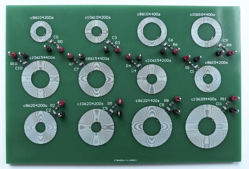
Sensor Resonant Frequency Results#
As mentioned earlier, the resonant frequency is a function of inductance and total capacitance. There’s technically an infinite number of L–C combinations that produce the same resonant frequency, so with my current test setup, comparing this frequency should be enough to indicate whether my approximation is on the right track.
| Coil Name | Resonant Frequency Approximation | TI Resonant Frequency | Measured Resonant Frequency | Error Percentage [Approx, TI] |
|---|---|---|---|---|
| C106102200s | 2.472E+06 | 2.743E+06 | 2.504E+06 | 1.27% 9.57% |
| C106152200s | 1.581E+06 | 1.729E+06 | 1.585E+06 | 0.26% 9.06% |
| C106202200s | 1.142E+06 | 1.236E+06 | 1.127E+06 | 1.26% 9.63% |
| C106102400s | 1.871E+06 | 2.012E+06 | 1.845E+06 | 1.44% 9.07% |
| C106152400s | 1.231E+06 | 1.316E+06 | 1.220E+06 | 0.95% 7.90% |
| C106202400s | 910.547E+03 | 970.507E+03 | 886.300E+03 | 2.74% 9.50% |
| C106104200s | 1.254E+06 | 1.424E+06 | 1.245E+06 | 0.69% 14.36% |
| C106154200s | 789.467E+03 | 885.439E+03 | 787.500E+03 | 0.25% 12.44% |
| C106204200s | 568.526E+03 | 631.114E+03 | 558.800E+03 | 1.74% 12.94% |
| C106104400s | 949.397E+03 | 1.046E+06 | 922.300E+03 | 2.94% 13.41% |
| C106154400s | 614.966E+03 | 673.882E+03 | 604.200E+03 | 1.78% 11.53% |
| C106204400s | 453.639E+03 | 495.275E+03 | 438.000E+03 | 3.57% 13.08% |
| C106104200p | 2.508E+06 | 2.489E+06 | 0.74% | |
| C106154200p | 1.579E+06 | 1.561E+06 | 1.18% | |
| C106204200p | 1.137E+06 | 1.095E+06 | 3.85% | |
| C106104400p | 1.899E+06 | 1.827E+06 | 3.91% | |
| C106154400p | 1.230E+06 | 1.182E+06 | 4.06% | |
| C106204400p | 907.278E+03 | 857.600E+03 | 5.79% |
Table 6: Resonant Frequency Comparisons
Trace Resistance results#
| Coil Name | Calculated Trace Resistance | Measure Trace Resistance | Error % |
|---|---|---|---|
| C106102200s | 0.981 | 1.2060 | 18.64% |
| C106152200s | 1.472 | 2.1628 | 31.95% |
| C106202200s | 1.962 | 3.4518 | 43.15% |
| C106102400s | 1.598 | 1.7400 | 8.17% |
| C106152400s | 2.397 | 2.9600 | 19.03% |
| C106202400s | 3.196 | 4.7176 | 32.26% |
| C106104200s | 2.894 | 4.9500 | 41.55% |
| C106154200s | 4.340 | 8.9567 | 51.54% |
| C106204200s | 5.787 | 13.9600 | 58.55% |
| C106104400s | 4.712 | 7.1821 | 34.39% |
| C106154400s | 7.068 | 12.6993 | 44.34% |
| C106204400s | 9.424 | 18.3724 | 48.71% |
| C106104200p | 0.723 | 0.9898 | 26.92% |
| C106154200p | 1.085 | 1.7610 | 38.38% |
| C106204200p | 1.447 | 2.8085 | 48.49% |
| C106104400p | 1.178 | 1.4821 | 20.52% |
| C106154400p | 1.767 | 2.7888 | 36.64% |
| C106204400p | 2.356 | 3.7942 | 37.90% |
Table 7: Trace Resistance Comparison
Source of Error#
Parasitic Capacitance#
The method I used to approximate the parasitic capacitance isn’t quite right. As mentioned above, the coil has a voltage gradient — but the most significant potential difference is in the outer rings of a two-layer board, and on 4-layer boards the potential alternates between outer and inner rings as you transition between layers.
A method described in this post [6] could be used to measure both inductance and parasitic capacitance, but ultimately an impedance analyzer would be the best tool for the job.
Trace Resistance#
I was somewhat surprised by the trace resistance results — measured values were consistently higher than predicted. Two separate issues could be at play here, possibly compounding.
A. Cumulative error between the voltmeter and ammeter. If the ammeter reads high and the voltmeter reads low, the calculated resistance comes out higher than reality. B. Manufacturing tolerances. If the trace’s actual height and width were smaller than the design value, the resistance would come out higher than the calculation predicts.
Conclusion#
The approximation held up reasonably well, with consistent alignment across coil configurations. If I were to do this again, I’d vary trace width and spacing more, to see how those affect parasitic capacitance.
Resonant Frequency#
The approximation produced accurate results compared to measurement — in fact, significantly closer than the TI Coil Designer’s values. I can’t explain why the two approximations differ so much without more information about how TI computes its values. I know the self-inductances are being approximated with the same equation, and there’s still a discrepancy, so I suspect the main difference is in how physical dimensions are calculated.
Parallel Configuration#
Wiring the PCI in parallel didn’t show much advantage. Comparing similar inductance values between a 2-layer and 4-layer board, the difference was about 1 \(\Omega\). I’ll be looking into this more when I start testing how the coils respond to conductive targets.
Citation#
[1]Liu, T., Wei, Z., Chi, H., & Yin, B. (2019). Inductance Calculation of Multilayer Circular Printed Spiral Coils. Journal of Physics: ConferenceSeries, 1176, 062045. doi:10.1088/1742-6596/1176/6/062045
[2]Ulvr, M. (2018). Design of PCB search coils for AC magnetic flux density measurement. AIP Advances, 8(4), 047505. doi:10.1063/1.4991643
[3]Mohan, S., Hershenson, M., Boyd, S., Lee, T. (1999). Simple Accurate Expressions for Planar Spiral Inductances. IEEE JOURNAL OF SOLID-STATE CIRCUITS, VOL. 34, NO. 10
[4]Oberhauser, C. (2019). LDC Sensor Design. Texas Instruments White Paper